سیستم های کنترل خطی
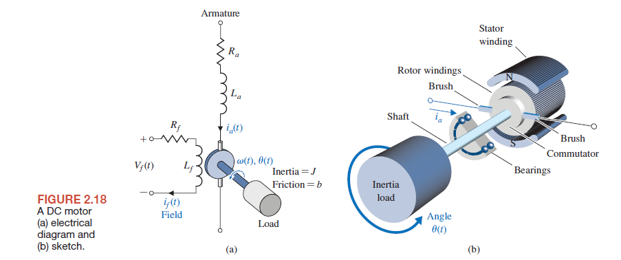
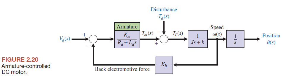
2)DC مدل موتور
.
.
مثال:
مثال 13-2 از کتاب سیستم های مدرن کنترل(دورف)
.
.
.
.
.
کد برنامه:
.
%DC Motor System Modeling and Analysis
clc; clear; close all;
%Page 135 (Dorf 14th edition)
% Define system parameters
Ra=1; % Armature resistance
La=1; % Armature inductance
J=2; % Moment of inertia
B=0.5; % Damping coefficient
Km=10; % Motor constant
Kb=0.1; % Back EMF constant
% Define the transfer functions for different parts of the system
num_G1=[Km]; den_G1=[La Ra]; G1=tf(num_G1,den_G1); % Transfer function for the motor
num_G2=[1]; den_G2=[J B]; G2=tf(num_G2,den_G2); % Transfer function for the mechanical system
num_G3=[1]; den_G3=[1 0]; G3=tf(num_G3,den_G3); % Transfer function for the integrator
num_G4=[Kb]; den_G4=[1]; G4=tf(num_G4,den_G4); % Transfer function for the back EMF
% Calculate the transfer functions of G11=y1/u1=teta/Va and G21=y2/u1=speed/Va
G1G2=series(G1,G2); % Combine the motor and mechanical system in series
G21=feedback(G1G2,G4) % Transfer function for the speed response to input voltage
G11=series(G21,G3) % Transfer function for the position response to input voltage
% Calculate the transfer functions of G12=y1/u2=teta/-Td and G22=y2/u2=speed/-Td
G1G4=series(G1,G4); % Combine the motor and back EMF in series
G22=feedback(G2,G1G4) % Transfer function for the speed response to load torque
G12=series(G22,G3) % Transfer function for the position response to load torque
.
.
3)DC اثر ورودی پله در موتور
.
برای دیدن اثر ورودی در خروجی موتور بخش زیر را به کد بالا اضافه کنید:
.
% Define the time range for the simulation
t0=0 ; tfinal=50; n=1000; t=linspace(t0,tfinal,n);
% Simulate the step response of the system for each transfer function
[y11,t11]=step(G11,t); % Step response for G11
[y12,t12]=step(G12,t); % Step response for G12
[y21,t21]=step(G21,t); % Step response for G21
[y22,t22]=step(G22,t); % Step response for G22
% Plot the step response of the system
subplot(2,2,1)
plot(t11,y11) % Plot the step response for G11
title('DC Motor Output');
xlabel('Time (seconds)') ;
ylabel('Angle(Rad)')
grid on
hold on
subplot(2,2,2)
plot(t12,y12) % Plot the step response for G12
title('DC Motor Output');
xlabel('Time (seconds)')
ylabel('Angle(Rad)')
grid on
hold on
subplot(2,2,3)
plot(t21,y21) % Plot the step response for G21
title('DC Motor Output');
xlabel('Time (seconds)')
ylabel('Speed')
grid on
hold on
subplot(2,2,4)
plot(t22,y22) % Plot the step response for G22
title('DC Motor Output');
xlabel('Time (seconds)')
ylabel('Speed')
grid on
hold on
.
.
4) PID , PI , P دیدن مکان هندسی ریشه ها با استفاده از کنترل کننده های
4-1)P کنترل کننده
.
کد برنامه:
.
% DC Motor Control (P)
clc; clear; close all;
% Define system parameters
Ra=1; % Armature resistance
La=1; % Armature inductance
J=2; % Moment of inertia
B=0.5; % Damping coefficient
Km=10; % Motor constant
Kb=0.1; % Back EMF constant
% Define the proportional controller
F=1; % C(s)=K*F(s) C(s) = Kp
% Define the transfer functions for different parts of the system
num_G1=[Km]; den_G1=[La Ra]; G1=tf(num_G1,den_G1); % Transfer function for the motor
num_G2=[1]; den_G2=[J B]; G2=tf(num_G2,den_G2); % Transfer function for the mechanical system
num_G3=[1]; den_G3=[1 0]; G3=tf(num_G3,den_G3); % Transfer function for the integrator
num_G4=[Kb]; den_G4=[1]; G4=tf(num_G4,den_G4); % Transfer function for the back EMF
% Calculate the transfer functions of G11=y1/u1=teta/Va and G21=y2/u1=speed/Va
G1G2=series(G1,G2); % Combine the motor and mechanical system in series
G21=feedback(G1G2,G4); % Transfer function for the speed response to input voltage
G11=series(G21,G3); % Transfer function for the position response to input voltage
% Calculate the transfer functions of G12=y1/u2=teta/-Td and G22=y2/u2=speed/-Td
G1G4=series(G1,G4); % Combine the motor and back EMF in series
G22=feedback(G2,G1G4); % Transfer function for the speed response to load torque
G12=series(G22,G3); % Transfer function for the position response to load torque
% Speed control
% Plot the root locus of the system with the proportional controller
figure;
% Subplot for G11
subplot(2,2,1);
rlocus(F*G11);
title('Root Locus of G11');
grid on;
% Subplot for G12
subplot(2,2,2);
rlocus(F*G12);
title('Root Locus of G12');
grid on;
% Subplot for G21
subplot(2,2,3);
rlocus(F*G21);
title('Root Locus of G21');
grid on;
% Subplot for G22
subplot(2,2,4);
rlocus(F*G22);
title('Root Locus of G22');
grid on;
.
.
4-2)PI کنترل کننده
.
کد برنامه:
.
% DC Motor Control (PI)
clc; clear; close all;
% Define system parameters
Ra=1; % Armature resistance
La=1; % Armature inductance
J=2; % Moment of inertia
B=0.5; % Damping coefficient
Km=10; % Motor constant
Kb=0.1; % Back EMF constant
Ti=1; % Time constant of the integral part of the PI controller
% Define the PI controller transfer function
% The numerator coefficients [Ti 1] and the denominator coefficients [Ti 0]
% represent the equation F(s) = (Ti*s + 1) / (Ti*s)
% This corresponds to the standard form of a PI controller: F(s) = Kp + Ki/s,
% where Kp=1 (proportional gain) and Ki=1/Ti (integral gain)
F=tf([Ti 1],[Ti 0]);
% Define the transfer functions for different parts of the system
num_G1=[Km]; den_G1=[La Ra]; G1=tf(num_G1,den_G1); % Transfer function for the motor
num_G2=[1]; den_G2=[J B]; G2=tf(num_G2,den_G2); % Transfer function for the mechanical system
num_G3=[1]; den_G3=[1 0]; G3=tf(num_G3,den_G3); % Transfer function for the integrator
num_G4=[Kb]; den_G4=[1]; G4=tf(num_G4,den_G4); % Transfer function for the back EMF
% Calculate the transfer functions of G11=y1/u1=teta/Va and G21=y2/u1=speed/Va
G1G2=series(G1,G2); % Combine the motor and mechanical system in series
G21=feedback(G1G2,G4); % Calculate the transfer function for the speed response to input voltage
G11=series(G21,G3); % Calculate the transfer function for the position response to input voltage
% Calculate the transfer functions of G12=y1/u2=teta/-Td and G22=y2/u2=speed/-Td
G1G4=series(G1,G4); % Combine the motor and back EMF in series
G22=feedback(G2,G1G4); % Calculate the transfer function for the speed response to load torque
G12=series(G22,G3); % Calculate the transfer function for the position response to load torque
% Speed control
% Plot the root locus of the system with the PI controller
figure;
% Subplot for G11
subplot(2,2,1);
rlocus(F*G11);
title('Root Locus of G11');
grid on;
% Subplot for G12
subplot(2,2,2);
rlocus(F*G12);
title('Root Locus of G12');
grid on;
% Subplot for G21
subplot(2,2,3);
rlocus(F*G21);
title('Root Locus of G21');
grid on;
% Subplot for G22
subplot(2,2,4);
rlocus(F*G22);
title('Root Locus of G22');
grid on;
.
.
4-3)PID کنترل کننده
.
کد برنامه:
.
% DC Motor Control (PID)
clc; clear; close all;
% Define system parameters
Ra=1; % Armature resistance
La=1; % Armature inductance
J=2; % Moment of inertia
B=0.5; % Damping coefficient
Km=10; % Motor constant
Kb=0.1; % Back EMF constant
% Discrete-time PID controller with a derivative filter
Ti=1; % Time constant of the integral part of the PID controller
Td=2; % Time constant of the derivative part of the PID controller
T=0.5; % Sampling period
% Define the PID controller transfer function
% The numerator coefficients [Ti*(T+Td) T+Ti 1] and the denominator coefficients [T*Ti Ti 0]
% represent the equation F(s) = (Ti*(T+Td)*s^2 + (T+Ti)*s + 1) / (T*Ti*s^2 + Ti*s)
% This corresponds to a discrete-time PID controller with a derivative filter: F(s) = Kp + Ki/s + Kd*s/(1+T*s)
F=tf([Ti*(T+Td) T+Ti 1],[T*Ti Ti 0]);
% Define the transfer functions for different parts of the system
num_G1=[Km]; den_G1=[La Ra]; G1=tf(num_G1,den_G1); % Transfer function for the motor
num_G2=[1]; den_G2=[J B]; G2=tf(num_G2,den_G2); % Transfer function for the mechanical system
num_G3=[1]; den_G3=[1 0]; G3=tf(num_G3,den_G3); % Transfer function for the integrator
num_G4=[Kb]; den_G4=[1]; G4=tf(num_G4,den_G4); % Transfer function for the back EMF
% Calculate the transfer functions of G11=y1/u1=teta/Va and G21=y2/u1=speed/Va
G1G2=series(G1,G2); % Combine the motor and mechanical system in series
G21=feedback(G1G2,G4); % Transfer function for the speed response to input voltage
G11=series(G21,G3); % Transfer function for the position response to input voltage
% Calculate the transfer functions of G12=y1/u2=teta/-Td and G22=y2/u2=speed/-Td
G1G4=series(G1,G4); % Combine the motor and back EMF in series
G22=feedback(G2,G1G4); % Transfer function for the speed response to load torque
G12=series(G22,G3); % Transfer function for the position response to load torque
% Speed control
% Plot the root locus of the system with the PID controller
figure;
% Subplot for G11
subplot(2,2,1);
rlocus(F*G11);
title('Root Locus of G11');
grid on;
% Subplot for G12
subplot(2,2,2);
rlocus(F*G12);
title('Root Locus of G12');
grid on;
% Subplot for G21
subplot(2,2,3);
rlocus(F*G21);
title('Root Locus of G21');
grid on;
% Subplot for G22
subplot(2,2,4);
rlocus(F*G22);
title('Root Locus of G22');
grid on;
.
.


دیدگاهها
هیچ نظری هنوز ثبت نشده است.